
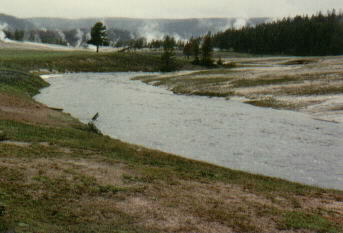
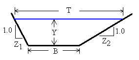
Photograph and Cross-Section of Trapezoidal Channel
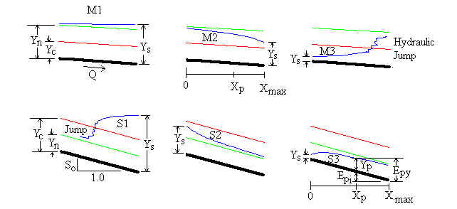
Gradually Varied Flow Profiles
Units: cm=centimeter, cfs=cubic feet per second, ft=feet, gal=US gallon, gpm=US gallons per minute,
gph=US gallons per hour, gpd=US gallons per day, km=kilometer, m=meter, MGD=Millions of US gallons per day, min=minute, s=second
Topics: Equations Variables Manning n Coefficients Error Messages References
Introduction
In long prismatic (constant cross-sectional geometry) channels, flowing water will attempt to reach the "normal depth" (also known as the "uniform flow depth"). Normal depth is the water depth determined using Manning's equation (please see our other web page for design of trapezoidal channels using Manning's equation). A gradually varied flow (GVF) profile is a plot of water depth versus distance along the channel as the water depth gradually achieves normal depth. A GVF computation in a trapezoidal channel involves starting at a known depth Ys and making successive water depth computations at small distance intervals. The method involves the continuity equation and energy slope equations. The LMNO Engineering calculation initially computes normal depth, critical depth, and GVF profile type. Then, it computes the water depth profile and plots it. The calculation also displays flow properties (depth, velocity, Froude number, etc.) at a specific location Xp entered by the user. A GVF profile is also known as a water depth profile, backwater calculation, and non-uniform flow computation. It is for steady state flows (discharge remains constant).
The LMNO Engineering calculation plots GVF profiles for M1, M2, S2, S3, C1, and C3 curves. M3 and S1 curves cross over the critical depth in order to achieve normal depth. Flows crossing the critical depth are called "rapidly varied flows" and cannot be computed using GVF methods.
Equations and Methodology
Fundamental flow equations are first presented, followed by equations for computing the critical depth Yc and normal depth Yn. Then, using the input value of Ys, the GVF profile type is determined and the GVF profile is computed using the Improved Euler method. References for the equations are shown alongside the equations. Manning's equation for Yn and the equation for the friction slope Sf are empirical; they are shown in the form that uses meters and seconds for units. Units for all other equations can be from any consistent set of units.
Fundamental Equations
The following equations are always valid for trapezoidal channels (Chanson, 1999; Chow, 1959; Simon and Korom, 1997):

Critical Depth Computation
To compute critical depth Yc the Froude number F is set to 1.0. Then, we use the Newton method (Kahaner, Moler, and Nash, 1989; Rao, 1985) along with the fundamental equations above to solve for Yc.
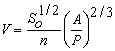
Normal Depth Computation
To compute normal depth Yn a cubic solution technique (Rao, 1985) is used to solve the fundamental equations above in conjunction with the Manning Equation (Chanson, 1999; Chaudhry, 1993; Chow, 1959; Simon and Korom, 1997):
Gradually Varied Flow Profile Determination
(Chanson, 1999; Chaudhry, 1993; Chow, 1959; Simon and Korom, 1997):
If Yn>Yc, then the channel is considered to have a
mild (M) slope. If Yn<Yc, the slope is steep
(S). If Yn=Yc, then the slope is termed critical (C).
The slopes are further classified by a number (1, 2, or 3) as follows:
For mild slopes (Yn>Yc):
If Ys>Yn, then the slope is an M1. The GVF
calculation starts downstream at Xmax at a depth of Ys
and proceeds upstream to X=0. The water depth gets closer to Yn
as the calculation proceeds further and further upstream.
If Yn>Ys >Yc, then the slope is an M2. The GVF calculation starts downstream at Xmax at a depth of Ys and proceeds upstream to X=0. The water depth gets closer to Yn as the calculation proceeds further and further upstream.
If Yc>Ys, then the slope is an M3. This is an unstable GVF calculation since the water depth begins below both Yn and Yc. Since the slope is mild, an hydraulic jump will occur. Hydraulic jumps are rapidly varied flow situations that cannot be modeled by a GVF calculator. Therefore, the message, "Cannot plot S1 or M3", will be shown.
For steep slopes (Yc>Yn):
If Ys>Yc, then the slope is an S1. This is an
unstable GVF calculation since the water depth begins above both Yc
and Yn. Since the slope is steep, the water depth will have to
pass through the critical depth in order to reach the normal depth. Passing through
the critical depth is a rapidly varied flow situation that cannot be modeled by a GVF
calculator. Therefore, the message, "Cannot plot S1 or M3", will be shown.
If Yc>Ys>Yn, then the slope is an S2. The GVF calculation starts upstream at X=0 at a depth of Ys and proceeds downstream to Xmax. The water depth gets closer to Yn as the calculation proceeds further and further downstream.
If Yn>Ys, then the slope is an S3. The GVF calculation starts upstream at X=0 at a depth of Ys and proceeds downstream to Xmax. The water depth gets closer to Yn as the calculation proceeds further and further downstream.
For critical slopes (Yc=Yn):
If Ys>Yc, then the slope is a C1. The GVF
calculation starts downstream at Xmax at a depth of Ys
and proceeds upstream to X=0. The water depth gets closer to Yn
as the calculation proceeds further and further upstream.
If Yc>Ys, then the slope is a C3. The GVF calculation starts upstream at X=0 at a depth of Ys and proceeds downstream to Xmax. The water depth gets closer to Yn as the calculation proceeds further and further downstream.
There is no such thing as a C2 slope - since Yc=Yn, Ys cannot be between Yc and Yn.
Gradually Varied Flow Profile (Graph) Computation
To compute the gradually varied flow profile (graph), the Improved Euler method (Chaudhry, 1993) is used:
At control section, i=1 and Yi=Ys.
Repeat for i=2 to n in increments of distance dX where dX
is negative for downstream control and dX is positive for upstream control.
Compute Ti, Ai, and Pi using the fundamental equations shown above using Y=Yi.
Compute the friction slope, depth increment, and intermediate depth (note: for the
friction slope equation shown, the friction slope variables must be in meters and
seconds):
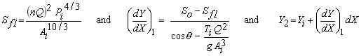
Compute T2, A2, and P2 using the fundamental equations shown above with Y=Y2. Then, compute the friction slope based on T2, A2, and P2 followed by computation of a second depth increment. Finally, compute the water depth, Yi+1 by using the average of the two differential depth increments (this is the basis of the Improved Euler method).
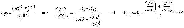
Then repeat the loop by incrementing i.
The LMNO Engineering calculation uses an unequal node spacing so that more nodes are used at the beginning of the calculation to improve accuracy. The first node spacing is approximately 10-10 m, and there are 4500 distance increments. The results have been checked against hand calculations, spreadsheets, and results shown in Chaudhry (1993), Chow (1959), French (1985), Henderson (1966), and Simon and Korom (1997).
Variables
Back to Calculation
Variables are shown below in SI units (metric). If you work through the above
equations by hand, use the SI units shown - since many of the equations are empirical and
are valid only with the indicated units. (The calculation
performs internal unit conversions which allow you to select a variety of different
units.)
A = Channel cross-sectional area [m2].
Ai = Area computed at successive i intervals in Improved Euler method [m2].
Ap = Area at Xp [m2].
A2 = Area for intermediate computation in Improved Euler method [m2].
dX = Distance increment for Improved Euler method [m]. Negative for M1, M2,
and C1 since computation proceeds upstream. Positive for S2, S3, and C3 since
computation proceeds downstream
(dY/dX)1 = First depth increment for Improved Euler method [m].
(dY/dX)2 = Second depth increment for Improved Euler method [m].
B = Channel bottom width [m].
E = Elevation [m]. The calculation automatically sets the channel invert
elevation to 0.0 at Xmax.
Epi = Elevation of channel invert at Xp [m].
Invert means bottom of the channel.
Epy = Elevation of water surface at Xp [m].
F = Froude number [dimensionless].
Fp = Froude number at Xp [dimensionless].
g = Acceleration due to gravity, 9.8066 m/s2.
i = Loop index for computing GVF profile.
n = Manning's n value [dimensionless]. See table below for
values.
P = Channel wetted perimeter [m].
Pi = Wetted perimeter computed at successive i intervals in Improved
Euler method [m].
P2 = Second wetted perimeter computed in Improved Euler method [m].
Q = Discharge (flowrate) of water in the channel [m3/s].
So = Slope of bottom of channel (vertical to horizontal ratio) [m/m].
Sf1 = First energy slope for Improved Euler method [dimensionless].
Sf2 = Second energy slope for Improved Euler method [dimensionless].
T = Top width of water in channel [m].
Ti = Top width computed at successive i intervals in Improved Euler
method [m].
T2 = Second top width computed in Improved Euler method [m].
Tp = Top width at Xp [m].
V = Average velocity of water [m/s].
Vp = Velocity at Xp [m/s].
X = Distance along channel [m].
Xmax = Maximum distance for computing GVF profile [m]. Profile is
always plotted from X=0 to Xmax. For M1, M2, and C1
profiles, Ys is at X=Xmax. For S2, S3, and
C3 profiles, Ys is at X=0.
Xp = Distance entered by user for showing channel properties [m].
Cannot exceed Xmax. If user enters Xp>Xmax,
the calculation will automatically set Xp to Xmax.
Y = Water depth [m].
Yc = Critical depth [m].
Yi = Water depth computed at successive i intervals in Improved Euler
method [m].
Yn = Normal depth [m].
Yp = Depth at Xp [m].
Ys = Starting depth [m]. This is also known as the depth at the
control section. It is the depth that GVF calculations start at.
Y2 = Second depth computed in Improved Euler method [m].
Z1 = One channel side slope (horizontal to vertical ratio) [m/m].
Z2 = The other channel side slope (horizontal to vertical ratio) [m/m].
Manning n Coefficients
Back to Calculation
The Manning's n coefficients were compiled from Chaudhry (1993), Chow (1959), French (1985), and Mays (1999).
| Material | Manning n | Material | Manning n |
| Natural Streams | Excavated Earth Channels | ||
| Clean and Straight | 0.030 | Clean | 0.022 |
| Major Rivers | 0.035 | Gravelly | 0.025 |
| Sluggish with Deep Pools | 0.040 | Weedy | 0.030 |
| Stony, Cobbles | 0.035 | ||
| Metals | Floodplains | ||
| Brass | 0.011 | Pasture, Farmland | 0.035 |
| Cast Iron | 0.013 | Light Brush | 0.050 |
| Smooth Steel | 0.012 | Heavy Brush | 0.075 |
| Corrugated Metal | 0.022 | Trees | 0.15 |
| Non-Metals | |||
| Glass | 0.010 | Finished Concrete | 0.012 |
| Clay Tile | 0.014 | Unfinished Concrete | 0.014 |
| Brickwork | 0.015 | Gravel | 0.029 |
| Asphalt | 0.016 | Earth | 0.025 |
| Masonry | 0.025 | Planed Wood | 0.012 |
| Unplaned Wood | 0.013 | ||
Error Messages
Back to Calculation
Initial Input Checks
The following messages are generated from improper input values:
"Need 1e-20<Q<1e50 m3/s", "Need 1e-20<B<1e6
m", "Need Z1, Z2 ≥0", "Z1, Z2
cannot both be 0", "Need 1e-9<n<20", "Need 1e-20<So<1e99",
"Need 0.001<Xmax<1e6 m", "Need 1e-20<Ys<100
m", "Need Xp≥0".
Run-Time Messages
The following messages may be generated during execution:
"Infeasible input". Inputs are unusually large or small causing
the program to have trouble computing Yn or Yc.
"Cannot plot S1 or M3". As discussed
above, these two GVF profiles encounter rapidly varied flow where the water depth
crosses through critical depth.
"No graph. Ys=Yn". This is a uniform flow
situation, not a GVF calculation. Water depth will remain at normal depth, so the
GVF profile is not computed. One would expect this message to occur if Yn is copied into the Ys field. However, the message may not appear since Yn is shown to only 8 significant figures but is stored internally to 18 significant figures.
"Yn at x=874.231 m". This is the distance where the
water depth is within 0.01% of the normal depth.
References
Back to Calculation
Chanson, H. 1999. The Hydraulics of Open Channel Flow. John Wiley and Sons, Inc.
Chaudhry, M. H. 1993. Open-Channel Flow. Prentice-Hall, Inc.
Chow, V. T. 1959. Open-Channel Hydraulics. McGraw-Hill, Inc. (the classic text)
French, R. H. 1985. Open-Channel Hydraulics. McGraw-Hill Book Co.
Henderson, F. M. 1966. Open Channel Flow. MacMillan Publishing Co.
Kahaner, D, C. Moler, and S. Nash. 1989. Numerical Methods and Software. Prentice-Hall, Inc. 2ed.
Mays, L. W. editor. 1999. Hydraulic design handbook. McGraw-Hill Book Co.
Rao, S. 1985. Optimization: Theory and Applications. Wiley Eastern Limited. 2ed.
Simon, A. and S. Korom. 1997. Hydraulics. Prentice-Hall, Inc. 4ed.
© 2001-2026 LMNO Engineering, Research, and Software, Ltd. All rights reserved.
LMNO Engineering, Research, and Software, Ltd.
7860 Angel Ridge Rd. Athens, Ohio 45701 USA Phone: (740) 707‑2614
LMNO@LMNOeng.com
https://www.LMNOeng.com