
Units: bbls/day=barrels/day (1 bbl=42 US gallons), cfm=ft3/min, cfs=ft3/s, cm=centimeter, cP=centipoise, cSt=centistoke, inch H2O=inch water at 60F, inch Hg=inch mercury at 60F, ft=foot, ft H2O= ft water at 60F, g=gram, gpd=gallon (US)/day, gph=gallon (US)/hr, gpm=gallon (US)/min, hp=horsepower, hr=hour, kg=kilogram, km=kilometer, lb=pound, m=meter, mbar=millibar, mm=millimeter, mm Hg=mm mercury at 0C, min=minute, N=Newton, Pa=Pascal (1 Pa=1 N/m2), psf=lb/ft2, psi=lb/inch2, s=second
Topics: Piping Scenarios Equations and Methodology Variables Minor Loss Coefficients Error Messages References
Introduction
The pump curve calculator pipe flow program automatically intersects a system curve with a pump curve to indicate the operating point. If you have a pump already installed or want to investigate system performance of a certain pump before purchasing it, enter two points on its pump curve along with piping system information to determine the flow rate through the system. Or, if you know the flow rate or velocity, you can solve for diameter, pipe length, pressure difference, elevation difference, or the sum of the minor loss coefficients.
A pump curve (blower curve for gases) is incorporated into the pump curve calculator to simulate systems containing a centrifugal pump or other pump that has a pump curve. To keep the calculator's input relatively simple, we only require you to enter two points on the pump curve - flow at zero head and head at zero flow. A parabolic curve is then formed between the two points as shown in equations below. The pump curve calculator also asks for information specifically about the pipe on the suction side of the pump. This information is used to compute the net positive suction head available (NPSHA) for liquids. For a pump to properly function, the NPSHA must be greater than the NPSH required by the pump (obtained from the pump manufacturer). If your system does not require a pump or uses a pump that does not have a parabolically shaped pump curve, then our other Darcy Weisbach design calculation may be more helpful.
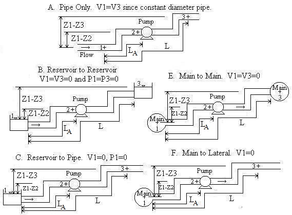
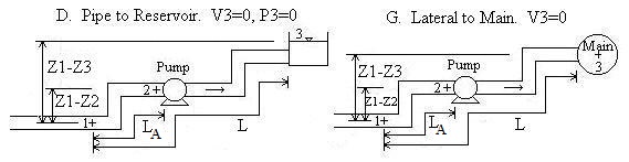
Piping Scenarios
Pipe A is the pipe upstream from the pump (i.e. the suction side pipe).
Convention for Z1-Z2 and Z1-Z3:
If location 1 is above location 2, then Z1-Z2 should be
entered as positive. If location 2 is above location 1, then Z1-Z2
should be entered as negative. Likewise for Z1-Z3.
Equations and Methodology Back to Calculation
The pump curve calculator uses the steady state incompressible energy equation. Minor losses (due to valves, pipe bends, etc.) and major losses (due to pipe friction) are included. The Darcy Weisbach equation for friction losses is used and the pump curve calculator includes both laminar and turbulent flow. The equations are standard equations which can be found in most fluid mechanics textbooks (see references below). A pump curve is included in the calculation. Determination of the pump curve requires that the user enter the two extreme points on the curve - head when flow is zero, and flow when head is zero. Then, a parabola with a negative curvature is fit through the two points. This parabola is used since it is a good approximation of a typical pump curve and does not require users to enter a multitude of data points. And, oftentimes, pump catalogs only give the two extreme points on the curve rather than a graph showing the complete curve.
Energy equation with Darcy-Weisbach friction losses
All equations were compiled from references except for parabolic
pump curve equation which is our development. The Colebrook equation is an equation
representation of the Moody diagram.
Pump Curve
To provide an example of a pump curve developed using the equation H=Hmax[1-(Q/Qmax)2],
let Qmax=1500 gpm (when head is zero) and Hmax=900 ft
(when Q is zero). The pump curve used in the calculation will look like:
The Colebrook equation is solved for f using Newton's method (Kahaner et al., 1989). The remaining calculations are analytic (i.e. closed form) except "Solve for V, Q", "Q known. Solve for Diameter", and "V known. Solve for Diameter". These three calculations required a numerical solution. Our solution utilizes a cubic solver (Rao, 1985) with the result accurate to 8 significant digits. Multiple solutions are possible for the three numerical solutions. All solutions for both laminar and turbulent flow are automatically determined and shown, if they exist. All of the calculations utilize double precision, but numbers are shown with six significant figures. The calculation does not check if velocities are unreasonable, such as gases flowing at over half the speed of sound which would require use of compressible gas equations.
Pump Curve Calculator Built-in fluid and material properties
You may enter fluid properties or select one of the common liquids or gases
from the drop-down menu. Weight density, kinematic viscosity, and vapor pressure (if
a liquid) for the built-in fluids were obtained from references.
Likewise, enter material roughness or select one of the common
pipe materials listed in the other drop-down menu. Surface roughnesses for the
built-in materials were compiled from references.
Net Positive Suction Head
NPSH is the sum of the heads that push fluid into a pump less the suction side
losses. Most pumps have a minimum requirement for NPSH, called NPSHR.
If the NPSH available by the piping system (NPSHA) is lower
than NPSHR, then the pump will not function properly and may overheat.
NPSH is only defined for liquids.
Variables Units: F=force,
L=length, P=pressure, T=time
Back to Calculation
Fluid density and viscosity may be entered into the pump curve calculator a wide choice of units. Some of the density units are mass density (g/cm3, kg/m3, slug/ft3, lb(mass)/ft3) and some are weight density (N/m3, lb(force)/ft3). There is no distinction between lb(mass)/ft3 and lb(force)/ft3 in the density since they have numerically equivalent values and all densities are internally converted to N/m3. Likewise, fluid viscosity may be entered in a wide variety of units. Some of the units are dynamic viscosity (cP, poise, N-s/m2 (same as kg/m-s), lb(force)-s/ft2 (same as slug/ft-s) and some are kinematic viscosity (cSt, stoke (same as cm2/s), ft2/s, m2/s). All viscosities are internally converted to kinematic viscosity in SI units (m2/s). If necessary, the equation Kinematic viscosity = Dynamic viscosity/Mass density is used.
A = Pipe inside cross-sectional area [L2]
D = Pipe inside diameter [L].
e = Pipe roughness [L].
f = Moody friction factor, used in Darcy-Weisbach friction loss equation.
g = Acceleration due to gravity = 32.174 ft/s2 = 9.8066 m/s2
hf = Major losses for entire pipe [L]. Also known as friction
losses.
hfA = Major losses for pipe upstream of pump (pipe A) only [L].
hm = Minor losses for entire pipe [L].
hmA = Minor losses for pipe upstream of pump (pipe A) only [L].
H = Total dynamic head [L]. Also known as system head or head supplied by
pump.
Hmax = Maximum head that pump can provide [L]. It is the head
when Q=0.
K = Sum of minor loss coefficients for entire pipe. See table below for values.
KA = Sum of minor loss coefficients for pipe upstream of pump (pipe
A). Same as Ka. Only required for liquids.
L = Total pipe length [L].
LA = Length of pipe upstream of pump (pipe A) [L]. Same as La.
Only required for liquids.
NPSH = Net positive suction head [L]. The calculation computes NPSHA
(NPSH available).
Patm = Atmospheric (or barometric) pressure [P]. Standard
atmospheric pressure = 14.7 psi = 29.92 inch Hg = 760 mm Hg = 1 atm = 101,325 Pa = 1.01
bar. Note that your local atmospheric pressure is different from standard
atmospheric pressure. Be careful - if you change the units of Patm and Pv, be sure
to enter Patm in the selected units. Only required for liquids.
Pv = Vapor pressure of fluid [P]. Expressed as an absolute
pressure. Only required for liquids.
P1 = Gage pressure at location 1 of the system [P]. Location 1
could be the surface of a reservoir open to the atmosphere (thus P1=0),
or the pressure in a supply main (same as a tank under pressure), or location 1 could
simply be a location in a pipe upstream of the pump. Only required for liquids.
P1-P3 = Pressure difference between locations 1 and 3 [P].
Q = Flowrate [L3/T]. Also known as discharge or capacity.
Qmax = Maximum flowrate on pump curve [L3/T].
Corresponds to point on pump curve where head is zero.
Re = Reynolds number.
S = Specific weight of fluid (i.e. weight density; weight per unit volume) [F/L3].
Typical units are N/m3 or lb(force)/ft3. Note that
S=(mass density)(g)
V1 = Velocity of fluid at location 1. This is determined when
a scenario is selected. If location 1 is a reservoir or main (Scenarios B, C, E, and
F), then V1 is automatically set to 0 because the velocity head of the
fluid in the reservoir or main (or pressure tank) is much smaller than in the attached
pipeline. This is a standard assumption in fluid mechanics. However, if
location 1 is inside the suction side pipeline, then V1 is
automatically computed as Q/A.
V3 = Velocity of fluid at location 3. This is determined when
a scenario is selected. If location 3 is a reservoir or main (Scenarios B, D, E, and
G), then V3 is automatically set to 0 because the velocity head of the
fluid in the reservoir or main (or pressure tank) is much smaller than in the attached
pipeline. This is a standard assumption in fluid mechanics. However, if
location 3 is inside your discharge side pipeline, then V3 is
automatically computed as Q/A.
Z1-Z2 = Elevation of location 1 minus elevation of pump
[L]. If the pump is above location 1, then enter this value as negative. Only
required for liquids.
Z1-Z3 = Elevation of location 1 minus elevation of location
3 [L].
v = Kinematic viscosity of fluid [L2/T]. Greek letter
"nu". Note that kinematic viscosity is equivalent to dynamic (or absolute)
viscosity divided by mass density. Mass density=S/g.
Table of Minor Loss Coefficients (K
is unit-less)
Back to Calculation
Compiled from references
| Fitting | Km | Fitting | Km |
| Valves: | Elbows: | ||
| Globe, fully open | 10 | Regular 90°, flanged | 0.3 |
| Angle, fully open | 2 | Regular 90°, threaded | 1.5 |
| Gate, fully open | 0.15 | Long radius 90°, flanged | 0.2 |
| Gate 1/4 closed | 0.26 | Long radius 90°, threaded | 0.7 |
| Gate, 1/2 closed | 2.1 | Long radius 45°, threaded | 0.2 |
| Gate, 3/4 closed | 17 | Regular 45°, threaded | 0.4 |
| Swing check, forward flow | 2 | ||
| Swing check, backward flow | infinity | Tees: | |
| Line flow, flanged | 0.2 | ||
| 180° return bends: | Line flow, threaded | 0.9 | |
| Flanged | 0.2 | Branch flow, flanged | 1.0 |
| Threaded | 1.5 | Branch flow, threaded | 2.0 |
| Pipe Entrance (Reservoir to Pipe): | Pipe Exit (Pipe to Reservoir) | ||
| Square Connection | 0.5 | Square Connection | 1.0 |
| Rounded Connection | 0.2 | Rounded Connection | 1.0 |
| Re-entrant (pipe juts into tank) | 1.0 | Re-entrant (pipe juts into tank) | 1.0 |
Error Messages
Back to Calculation
The following are input checks and will appear if an input is physically impossible, such
as a negative length. Some or all values may be computed even with error messages, even though physically the situation cannot occur.
"Q, V, D, L must be > 0", "Density, Viscosity must be > 0",
"K must be ≥ 0", "e must be ≥ 0", "Qmax , Hmax
must be > 0", "Q must be ≤ Qmax".
The following are messages for liquids only:
"La, Ka must be ≥ 0", "Vapor and Atm P
must be > 0".
"Need La ≤ L and Ka ≤ K". Length of the
suction pipe (Pipe A) was entered as being longer than all of the pipe, or K for the
suction pipe was entered as greater than K for the entire system.
"P1+Patm must be >0." The sum of P1+Patm
gives P1 in absolute pressure. It is physically impossible to
have an absolute pressure ≤ 0 since that implies a complete vacuum at location 1.
"Need P1-(P1-P3)+Patm >0."
The absolute pressure at location 3 is less than 0 absolute. It is physically impossible to have a complete vacuum.
Other messages:
"K must be ≥ 1". If "Q known. Solve for D" and V3=0,
then K must be > 1 in order to solve.
"Tanks open, so P1-P3=0 for B". Cannot solve
for pressure difference if using Scenario B since reservoirs are defined to be at
zero pressure thus zero pressure difference.
"Infeasible input. H<0", "Infeasible input. hm<0",
"Infeasible input. hf ≤0", "Re or e/D out of range",
"Infeasible. Losses will be ≤0", "f won't be 0.008 to 0.1",
"f will be too small", "f will be too large", "Re will be >
1e8", "Infeasible input". One of these messages will appear if
each of your inputs is okay, but they combine to give no possible solution. For
instance, if solving for pipe diameter and input data results in negative
losses regardless of pipe diameter, then input data are infeasible.
References
Back to Calculation
Numerical methods citations
Kahaner, D., C. Moler, and S. Nash. 1989. Numerical methods and software.
Prentice-Hall, Inc.
Rao, S. S. 1985. Optimization theory and applications. Wiley Eastern Limited. 2ed.
Fluid mechanics references
Gerhart, P. M, R. J. Gross, and J. I. Hochstein. 1992. Fundamentals of Fluid
Mechanics. Addison-Wesley Publishing Co. 2ed.
Mays, L. W. editor. 1999. Hydraulic design handbook. McGraw-Hill Book Co.
Munson, B.R., D. F. Young, and T. H. Okiishi. 1998. Fundamentals of Fluid Mechanics. John Wiley and Sons, Inc. 3ed.
Potter, M. C. and D. C. Wiggert. 1991. Mechanics of Fluids. Prentice-Hall, Inc.
Roberson, J. A. and C. T. Crowe. 1990. Engineering Fluid Mechanics. Houghton Mifflin Co.
Streeter, V. L., E. B. Wylie, and K. W. Bedford. 1998. Fluid Mechanics. WCB/McGraw-Hill. 9ed.
White, F. M. 1979. Fluid Mechanics. McGraw-Hill, Inc.
© 2001-2026 LMNO Engineering, Research, and Software, Ltd. All rights reserved.
LMNO Engineering, Research, and Software, Ltd.
7860 Angel Ridge Rd. Athens, Ohio 45701 USA Phone: (740) 707-2614
LMNO@LMNOeng.com
https://www.LMNOeng.com